FIR analysis exemple
How to perform theoretical analysis of a FIR filter ? We present here on an example such an anlysis.
We consider the following mean filter defined by the input-output equation $$ s[t] = \frac{1}{4}e[t-1] + \frac{1}{2}e[t]+ \frac{1}{4}e[t+1] $$ where $s[t]$ is the output and $e[t]$ the input.
Theoretical analysis
Basic analysis
The system is clearly linear (the output is simple linear combination of the input) and time-invariant (the linear combination is same for all $t$), so the input-output equation indeed corresponds to a filtering.
The system is a-causal as the output at time $t$ depends of the input at the time $t+1$ adn at the time $t$ and before.
Transfert function
The transfert function $H(z)$ can be obtained by applying the $z$-transform on the input-output equation and using the properties of the $z$-transform (in particular, the time shift properties) $$ \begin{aligned} S(z) & = \frac{1}{4}z^{-1} E(z)+ \frac{1}{2} E(z)+ \frac{1}{4} z E(z)\\ & = \left(\frac{1}{4}z^{-1} + \frac{1}{2}+ \frac{1}{4} z \right)E(z) \end{aligned} $$ then $$ H(z) = \frac{1}{4}z^{-1} + \frac{1}{2}+ \frac{1}{4} z $$ the region of convergence is $|z|\neq 0$, the filter being a-causal.
Stability
$1$ is in the region of convergence, then the filter is stable.
Impulse response
The impulse response is obtained simply by inversion of the $z$-transform, using the table and the time shift properties, or by using the Dirac as the input ($e[t]=\delta[t]$): $$ h[t] = \frac{1}{4}\delta[t-1] + \frac{1}{2}\delta[t] + \frac{1}{4} \delta[t+1] $$ that is $$ \begin{aligned} h[-1] & = \frac{1}{4} \\ h[0] & = \frac{1}{2} \\ h[1]& = \frac{1}{4}\\h[t]& =0\quad \text{ otherwise } \end{aligned} $$ We recover the stability of the system: $\Vert h \Vert_1 = \frac{1}{4}+\frac{1}{2}+\frac{1}{4} = 1 < +\infty$
Complex gain and frequency response
The complex gain is obtained from the transfert function: $$ \begin{aligned} \hat h(\nu) & = H(e^{i2\pi\nu}) = \frac{1}{4}e^{-i2\pi\nu} + \frac{1}{2}+ \frac{1}{4} e^{i2\pi\nu} \\ & = \frac{1}{2}\left(\frac{e^{-i2\pi\nu}+e^{-i2\pi\nu}}{2} +1 \right)\\ & = \frac{1}{2}(\cos(2\pi\nu)+1) \\ &= \cos^2(\pi\nu) \end{aligned} $$ The complex gain is real because the impulse response is symmetric.
The frequency response reads: $$ |\hat h(\nu)|^2 = \cos^4(\pi\nu) $$ The filter is then a low-pass filter.
Matlab simulation
Introduction: preparation
close all;clear;clc;
[x,fs] = audioread('string_1.mp3');
x = 0.5*x(:,1)+0.5*x(:,2);
T = length(x);
Filtering implementations
First implementation: a simple loop. The first and last coefficients must be computed separately. When the filter is causal, this implementation is compatible with real time
s1 = x;
s1(1) = 0.5*x(1) + 0.25*x(2);
s1(T) = 0.25*x(T-1) + 0.5*x(T);
for t=2:T-1
    s1(t) = 0.25 * x(t-1) + 0.5*x(t) + 0.25*x(t+1);
end
Second implementation: using vector operation. Should be must efficient that the previous one. Interesting for “batch” manipulation (no need of real time.
s2 = x;
s2(1) = 0.5*x(1) + 0.25*x(2);
s2(T) = 0.25*x(T-1) + 0.5*x(T);
s2(2:T-1) = 0.25*x(1:T-2) + 0.5*x(2:T-1) + 0.25*x(3:T);
We check that the two implementations lead to the same result
disp(norm(s1-s2,'inf'))
Third implementation: using the filter function and the impulse response h. the filter function suppose that the filter is causal. We need to proceed to a time shift to obtain the right result. The last coefficient must be computed separately
h = [0.25;0.5;0.25];
s3 = filter(h,1,x);
s3(1:T-1) = s3(2:T);
s3(T) = 0.25*x(T-1) + 0.5*x(T);
We check that the three implementations lead to the same result
disp(norm(s1-s3,'inf'))
Numerical analysis of the filter.
We first compute the frequency response of the filter
[H,W] = freqz(h,1,round(T/2),fs);
figure(1);
plot(W,20*log(abs(H)+eps));
title('Frequency response of the filter (in db)');
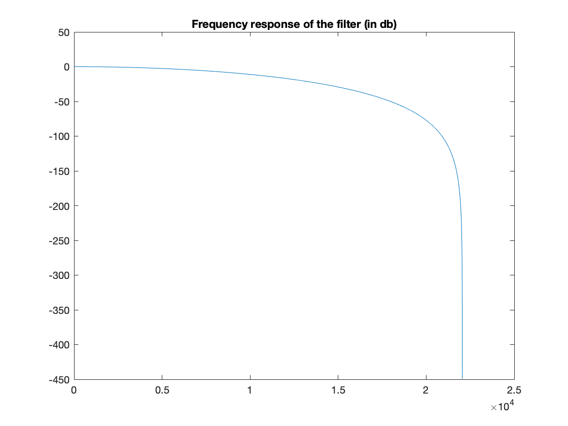
The filter is a low pass filter: an attenuation of frequencies about 25 db is attained around 15000 Hz.
We compare the spectrum of the input signal and the ouput signal. The signals are real, so we only display the positive frequencies
x_fft = fft(x);
x_spectrum_db = 20*log(abs(x_fft)+eps);

s_fft = fft(s1);
s_spectrum_db = 20*log(abs(s_fft)+eps);
The frequency axis is given in W. We could construct the axis as freq_axis = linspace(0,fs/2,round(T/2));
freq_axis = W;
figure(2);
plot(freq_axis,x_spectrum_db(1:round(T/2)),'r',freq_axis,s_spectrum_db(1:round(T/2)),'b');
title('Spectrum of the input and output signals (in db)');
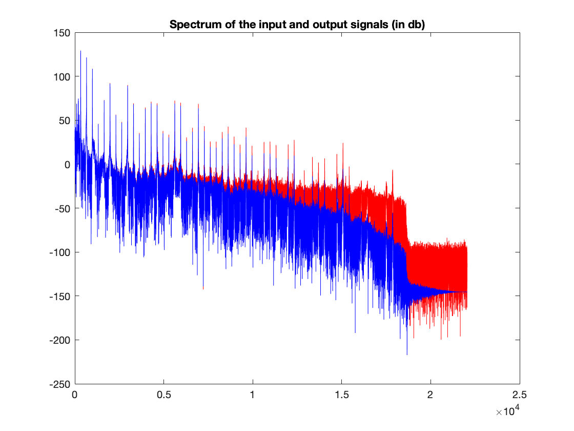
The compared spectrums confirm the low pass filter behavior.
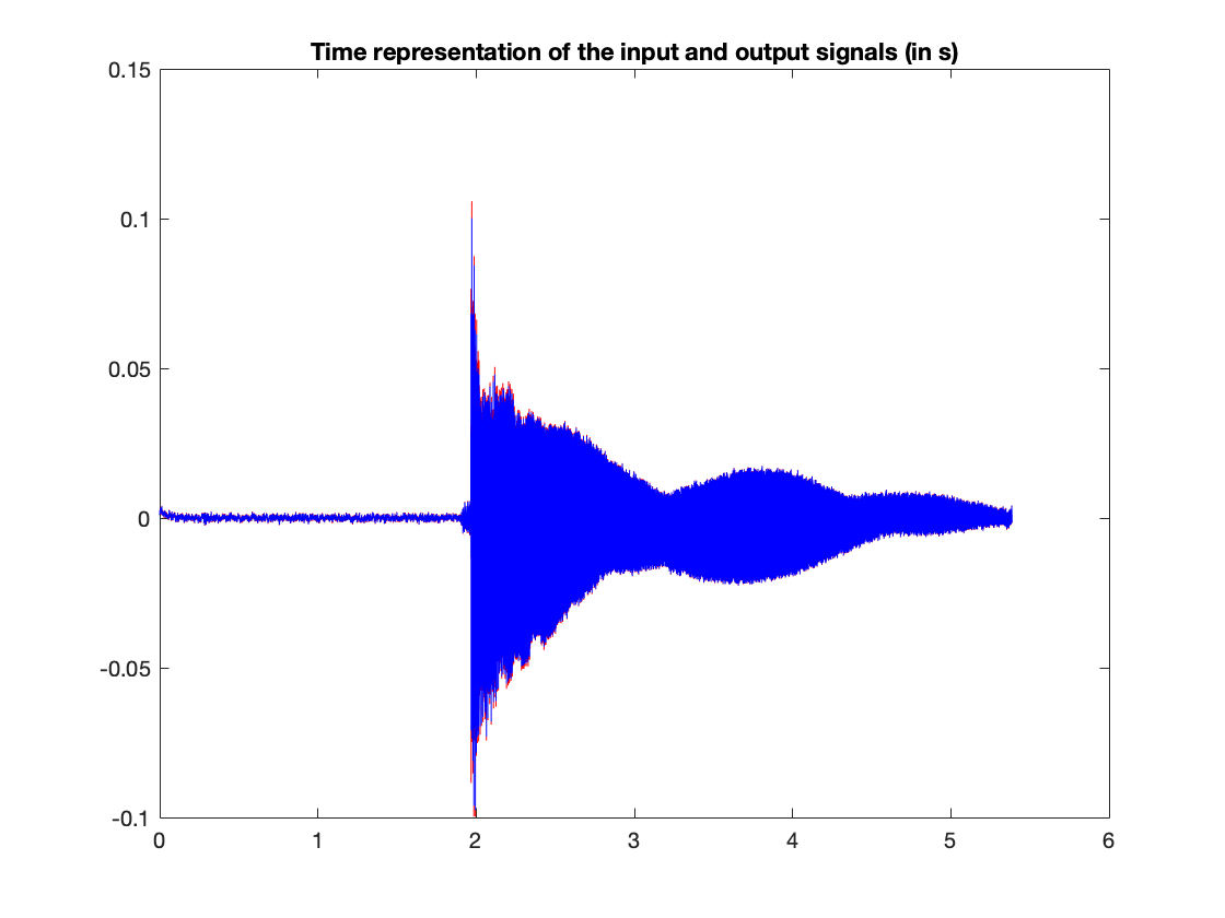
We compare the time signals
time_axis = linspace(0,T/fs,T);
figure(3)
plot(time_axis,x,'r',time_axis,s1,'b');
title('Time representation of the input and output signals (in s)');