IIR analysis exemple
How to perform theoretical analysis of an IIR filter ? We present here on an example such an analysis.
We consider the following mean filter defined by the input-output equation: $$ s[t] = \frac{1}{2}s[t-1]+4e[t]+2e[t-1] $$ where $s[t]$ is the output and $e[t]$ the input.
Theoretical analysis
Basic analysis
The system is clearly linear (the output is simple linear combination of the input and the previous values of the output) and time-invariant (the linear combination is same for all $t$), so the input-output equation indeed corresponds to a filtering.
The system is causal as the output at time $t$ depends of the input and the output the time $t$ and before.
Transfert function
The transfert function $H(z)$ can be obtained by applying the $z$-transform on the input-output equation and using the properties of the $z$-transform (in particular, the time shift properties) $$ \begin{aligned} S(z) & = \frac{1}{2}z^{-1} S(z)+ 4 E(z)+ 3z^{-1} E(z)\\ (1-\frac{1}{2}z^{-1})S(z) & = (4+3z^{-1}) E(z)\\S(z) & = \frac{4+3z^{-1}}{1-\frac{1}{2}z^{-1}} E(z) \end{aligned} $$ then $$ H(z) = \frac{4+3z^{-1}}{1-\frac{1}{2}z^{-1}} $$ the region of convergence is $|z|> \frac{1}{2}$, the filter being causal.
Stability
$1$ is inside the region of convergence, then the filter is stable
Impulse response
We perform a partial fraction decomposition of $H(z)$
$$ H(z) = 4\frac{1}{1-\frac{1}{2}z^{-1}} + 3\frac{z^{-1}}{1-\frac{1}{2}z^{-1}} $$ The impulse response is then obtained by inversion of the $z$-transform, using the table and the time shift properties: $$ \begin{aligned} h[t] & = 4 \cdot \frac{1}{2^t} \Theta[t] + 3 \cdot \frac{1}{2^{t-1}} \Theta[t-1]\\& = 4\delta[t] + 11 \cdot \frac{1}{2^{t-1}} \Theta[t-1] \end{aligned} $$
Complex gain and frequency response
The complex gain is obtained from the transfert function: $$ \begin{aligned} \hat h(\nu) & = H(e^{i2\pi\nu}) = \frac{4+3e^{-i2\pi\nu}}{1-\frac{1}{2}e^{-i2\pi\nu}} \end{aligned} $$
The frequency response reads: $$ \begin{aligned} |\hat h(\nu)|^2 & = \left|\frac{4+3e^{-i2\pi\nu}}{1-\frac{1}{2}e^{-i2\pi\nu}}\right|^2\\ & = \frac{(4+3\cos(2\pi\nu))^2+9\sin^2(2\pi\nu)}{(1-\frac{1}{2}\cos(2\pi\nu))^2+\frac{1}{4}\sin^2(2\pi\nu)}\\ &= \frac{25+24\cos(2\pi\nu)}{\frac{5}{4}-\cos(2\pi\nu)} \end{aligned} $$ The filter is then a low-pass filter.
Matlab simulation
Introduction: preparation
close all;clear;clc;
[x,fs] = audioread('string_1.mp3');
x = 0.5*x(:,1)+0.5*x(:,2);
T = length(x);
Filtering implementations
First implementation: a simple loop. The first coefficient must be computed separately. When the filter is causal, this implementation is compatible with real time
s1 = x;
s1(1) = 4*x(1);
for t=2:T
    s1(t) = 0.5*s1(t-1) + 4 * x(t) + 2*x(t-1) ;
end
Second implementation: using the filter function and the two impulse responses used to implement the IIR filter.
B = [4;2];
A = [1,-0.5];
s2 = filter(B,A,x);
We check that the two implementations lead to the same result
disp(norm(s1-s2,'inf'))
Numerical analysis of the filter.
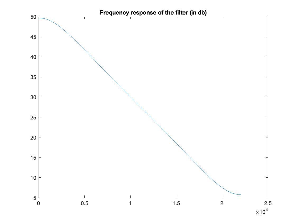
We first compute the frequency response of the filter
[H,W] = freqz(B,A,round(T/2),fs);

figure(1);
plot(W,20*log(abs(H)+eps));
title('Frequency response of the filter (in db)');
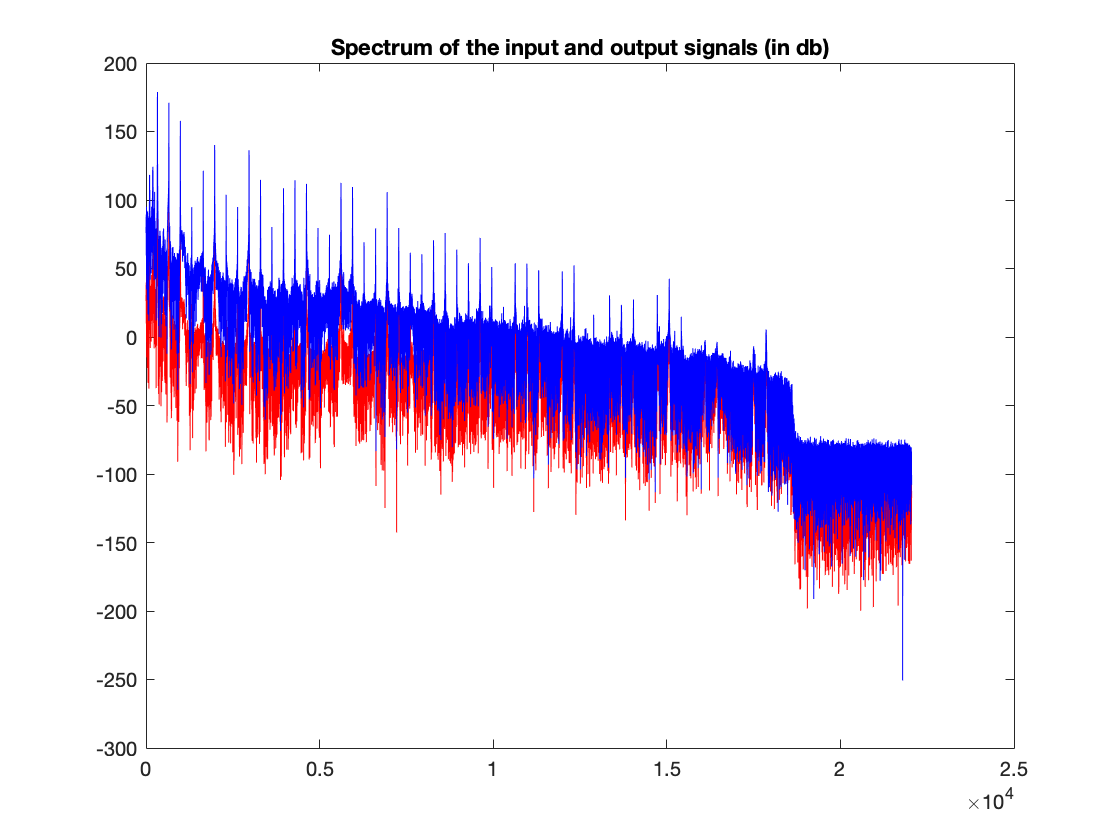
We compare the spectrum of the input signal and the ouput signal. The signals are real, so we only display the positive frequencies
x_fft = fft(x);
x_spectrum_db = 20*log(abs(x_fft)+eps);

s_fft = fft(s2);
s_spectrum_db = 20*log(abs(s_fft)+eps);
The positive frequencies axis is given in W.
freq_axis = W;
figure(2);
plot(freq_axis,x_spectrum_db(1:round(T/2)),'r',freq_axis,s_spectrum_db(1:round(T/2)),'b');
title('Spectrum of the input and output signals (in db)');
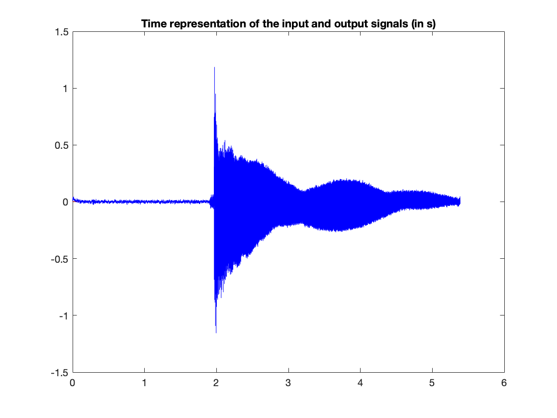
We compare the time signals
time_axis = linspace(0,T/fs,T);
figure(3)
plot(time_axis,x,'r',time_axis,s1,'b');
title('Time representation of the input and output signals (in s)');